Twenty-Five Stars and the Scale of the Universe

Updated 13 October 2026. The retrospective archive date and later literature are documented in the changelog.

On 3 March 1912, Harvard College Observatory issued a three-page circular about 25 variable stars in the Small Magellanic Cloud. Its table gives their brightnesses and periods. Its last page gives two graphs and Edward C. Pickering’s signature. Its first sentence says that the statement was prepared by Henrietta Leavitt [[1]].

That combination is worth keeping in view: the measurements, the inference, and the institution through which the result reached its readers.

The discovery is often compressed into a sentence about a woman who measured the universe. I would rather start with two columns in her table. The remarkable thing is how much follows from them, and exactly what does not.

Brightness Has a Distance Problem

A faint star can be intrinsically faint, far away, or both. Ignoring extinction for the moment, its observed flux is

$$ F = \frac{L}{4\pi d^2}, $$

where $L$ is luminosity, the energy emitted per unit time, $d$ is distance, and $F$ is energy received per unit area per unit time. For observations in a particular wavelength band, the corresponding band luminosity and band flux must be used consistently.

One brightness measurement gives one equation with two unknowns. A photograph does not resolve that ambiguity by being particularly beautiful.

Leavitt’s stars offered an unusually useful comparison. They belonged to the same apparent stellar system, the Small Magellanic Cloud. If their distances are approximately equal, a brighter member is approximately more luminous. The unknown common distance changes the absolute scale but preserves the brightness ranking. This is the argument made explicitly on the circular’s third page [[1]].

It is an approximation. A galaxy has depth. Dust can attenuate different sightlines by different amounts, and neighbouring stars can contaminate a measurement. Shared membership does not make those effects disappear. But it removes the largest obstacle to recognising an intrinsic relation: comparing unrelated stars scattered over a wide range of distances.

The Clock Is in the Star

A Cepheid is a pulsating star. Its radius and surface temperature change over a cycle, changing the amount and spectrum of light it emits. The period $P$ is the time taken to repeat that cycle. It can be estimated from a sequence of brightness measurements without first knowing the distance.

The underlying pulsation is driven by the opacity mechanism in partial ionisation layers of the stellar envelope. Around the region where helium becomes fully ionised, compression can increase opacity, temporarily impeding outward energy transport. The resulting pressure response can drive an oscillation. Whether a mode grows depends on the energy gained and lost over the whole cycle; the envelope also damps oscillations. This is why suitable stars occupy an instability strip, rather than every star pulsating visibly as a Cepheid [[2]].

There is a useful scale estimate behind the period. A self-gravitating star’s dynamical timescale is

$$ t_{\mathrm{dyn}} \sim \sqrt{\frac{R^3}{G\mathcal{M}}} \propto \bar\rho^{-1/2}, $$

where $R$ is radius, $\mathcal{M}$ is stellar mass, $G$ is the gravitational constant, and $\bar\rho$ is mean density. A radial pulsation period is related to this timescale, with a coefficient that depends on the star’s structure and pulsation mode. A larger, less dense star generally has a longer dynamical clock.

That estimate alone does not derive Leavitt’s law. Connecting the clock to luminosity also requires the relationships among mass, radius, temperature, and evolutionary state within the relevant stellar population. The relation was an empirical discovery before it was a fully developed stellar model.

This is the same distinction that matters in teaching stellar evolution: a mechanism can explain a tendency without making a short calculation into a complete model of a star.

What the Twenty-Five Rows Say

Leavitt had already remarked on the brightness–period pattern in her 1908 catalogue of 1,777 variables in the Magellanic Clouds. The 1912 circular developed the relation with 25 measured periods and graphs using both period and its logarithm. These are two stages of the discovery, rather than competing dates for a single moment [[1]] [[3]].

Here are the relevant columns of the original 1912 table. The magnitudes are on its provisional photographic scale. “Maximum” means maximum light, which has the smaller magnitude number [[1]].

Harvard Variable	Period / Days	Magnitude at Maximum Light	Magnitude at Minimum Light
1505	1.25336	14.8	16.1
1436	1.6637	14.8	16.4
1446	1.7620	14.8	16.4
1506	1.87502	15.1	16.3
1413	2.17352	14.7	15.6
1460	2.913	14.4	15.7
1422	3.501	14.7	15.9
842	4.2897	14.6	16.1
1425	4.547	14.3	15.3
1742	4.9866	14.3	15.5
1646	5.311	14.4	15.4
1649	5.323	14.3	15.2
1492	6.2926	13.8	14.8
1400	6.650	14.1	14.8
1355	7.483	14.0	14.8
1374	8.397	13.9	15.2
818	10.336	13.6	14.7
1610	11.645	13.4	14.6
1365	12.417	13.8	14.8
1351	13.08	13.4	14.4
827	13.47	13.4	14.3
822	16.75	13.0	14.6
823	31.94	12.2	14.1
824	65.8	11.4	12.8
821	127.0	11.2	12.1

The trend is visible without fitting anything. HV 1505 repeats in about 1.25 days and reaches magnitude 14.8; HV 821 takes 127 days and reaches 11.2. There is scatter, and a longer period does not make every neighbouring row brighter. The relation concerns a population trend.

In a calibrated magnitude system,

$$ m_1-m_2=-2.5\log_{10}\!\left(\frac{F_1}{F_2}\right). $$

A difference of 3.6 magnitudes would therefore correspond to a flux ratio of

$$ 10^{0.4(14.8-11.2)} \approx 27.5. $$

That gives the scale of the brightness contrast under the usual magnitude interpretation. It is not a precise flux measurement from these provisional photographic numbers. In particular, the historical plate response cannot simply be treated as a modern linear detector.

Why the Logarithm Straightens the Relation

Leavitt’s second graph uses $\log_{10}(P/\mathrm{day})$ on the horizontal axis. The two brightness sequences become approximately straight. Her stated trend was an increase of about 0.48 in log-period per magnitude of increased brightness, equivalent to a magnitude slope of approximately $-1/0.48=-2.08$ [[1]].

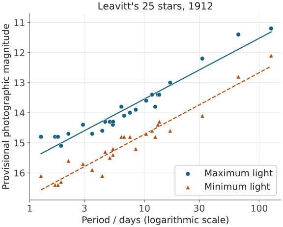
Reconstruction from the table above, with separate least-squares fits. The period axis is logarithmic; the magnitude axis is reversed so that brighter stars appear higher. The two measurements for each star are extrema, not uncertainty bounds.

For a reproducible descriptive check, I fitted each of the 25-row sequences with an unweighted least-squares line. This minimises the sum of squared vertical residuals in magnitude, treating the listed periods as exact inputs for this calculation. It gives

$$ m_{\mathrm{maximum\ light}} \approx 15.560-2.018\log_{10}(P/\mathrm{day}), $$$$ m_{\mathrm{minimum\ light}} \approx 16.766-2.049\log_{10}(P/\mathrm{day}). $$

These are my fits to the printed table, not coefficients reported by Leavitt. Their agreement with her approximate slope is the point of the reconstruction.

The midpoint of each pair of extrema gives another convenient demonstration:

$$ m_{\mathrm{mid}}\equiv \frac{m_{\mathrm{maximum\ light}}+m_{\mathrm{minimum\ light}}}{2} \approx 16.163-2.033\log_{10}(P/\mathrm{day}). $$

The residual root-mean-square, using all 25 stars and dividing the squared residual sum by 25, is approximately 0.224 magnitudes.

The midpoint is not the time-averaged magnitude. Cepheid light curves are asymmetric, so a star does not spend equal time at every brightness; averaging magnitudes also differs from averaging fluxes and then converting to a magnitude. Nor is 0.224 a measurement uncertainty assigned to each star. It is a descriptive scatter around this particular line, containing several physical and observational contributions.

In a calibrated band, a linear relation between magnitude and log-period corresponds to a power law between luminosity and period. But the historical fit’s slope and intercept are properties of this provisional dataset. They are not parameters to paste into a modern distance calculation.

The Missing Number Is the Zero Point

For a star observed in a specified band,

$$ m-M=5\log_{10}(d/10\,\mathrm{pc})+A, $$

where $m$ is apparent magnitude, $M$ is absolute magnitude—the magnitude the star would have at ten parsecs—and $A$ is extinction in that band.

Suppose the intrinsic relation is

$$ M=a\log_{10}(P/\mathrm{day})+b. $$

For stars at a common distance and with common extinction, the observed relation becomes

$$ m=a\log_{10}(P/\mathrm{day})+ \underbrace{b+5\log_{10}(d/10\,\mathrm{pc})+A}_{\text{observed intercept}}. $$

The slope can be found without knowing $d$. The intrinsic zero point $b$ cannot be separated from the distance contribution using these data alone. An independent distance is needed somewhere.

This is the crucial limit. Leavitt had found a way to recognise relative luminosities. Her 1912 circular did not establish an absolute distance scale in parsecs. Its request for parallaxes of brighter variables makes the need for additional measurements explicit. Also, its historical discussion of an “absolute scale of magnitudes” concerns standardising the photographic scale; it should not be mistaken for a completed determination of $M$ in the modern distance-modulus sense [[1]].

A simple hypothetical calculation shows what calibration adds. Suppose a calibrated relation assigns a star $M=-4$, and its extinction-corrected apparent magnitude is $m=21$. Then

$$ d=10^{(21-(-4)+5)/5}\,\mathrm{pc}=10^6\,\mathrm{pc}. $$

The distance is one megaparsec. Those numbers illustrate the method; they are not observations of one of Leavitt’s stars.

Even without the absolute zero point, two otherwise comparable Cepheids with the same period, observed in the same band, give a relative distance. If one is five extinction-corrected magnitudes fainter, it is ten times farther away. The clock supplies the comparison that an arbitrary pair of stars lacks.

A Useful Relation Still Needs Better Measurements

Modern astronomy has added calibrated photometry, much denser sampling, independent distance anchors, and corrections for composition, extinction, crowding, and the geometry of the stellar systems being compared. The classical-Cepheid relations also depend on wavelength and pulsation mode. There is no single universal brightness–period formula for every variable star [[2]] [[4]].

In the literature update of 13 October 2026, a 2025 reanalysis by Louise Breuval, Caroline Huang, and Adam Riess supplies a modern comparison. It returned to Leavitt’s sample and notebooks. They find good agreement between most historical and modern periods, but also a shallower historical brightness slope than expected for a modern blue band. They identify photographic non-linearity and crowding as likely contributors. Restricting the sample near the Small Magellanic Cloud’s centre reduces scatter. That is consistent with depth contributing to the scatter; a spatial cut alone does not isolate it from other differences between the retained and excluded stars [[3]].

That result is more interesting than declaring the old measurements perfect. The discovery survives, and the limitations of the apparatus remain visible.

The Cepheid rung of the cosmic distance ladder still uses this empirical connection. Geometric measurements calibrate Cepheids; Cepheids in suitable galaxies calibrate Type Ia supernovae; the supernovae extend the distance scale. Leavitt’s relation is essential to that route, but the geometric calibration comes first. Calling it the first rung without qualification conceals the missing zero point [[4]].

Measuring Plates Was Already Doing Science

The circular itself describes difficult conditions: crowded fields, faint stars, long exposures, and relatively few photographs. Recovering a period from those observations requires deciding how measurements taken on separate nights fit into a repeating cycle. Constructing comparable magnitudes requires comparison stars and a consistent scale. Identifying the relation requires choosing the comparison that makes the distance ambiguity manageable [[1]].

These decisions are intellectual work. The fact that much of it was performed at a desk, through repetitive measurement, does not make it merely preparatory to the science.

Harvard’s institutional histories describe a division of opportunity. Leavitt entered the observatory as a volunteer, supported by her family, and later held a paid position. Women employed as “computers” analysed photographic data, while access to observing and control over research questions were restricted. Leavitt’s work assignments also limited her freedom to continue the investigation she wanted [[5]] [[6]].

Recognition was not entirely absent within that arrangement. The Harvard–Smithsonian historical account reports that Leavitt was paid thirty cents an hour, five cents more than most computers. That comparison is with other computers, not with male astronomers doing an equivalent job. It shows that rewarding an individual’s skill and restricting her research authority could coexist [[5]].

That arrangement offered access to an extraordinary archive while limiting authority over what to do with it. Both parts matter. Opportunity within an unequal institution is not evidence that the inequality was harmless.

The family support matters too. Entry through unpaid work selects for people who can afford that entry. That is a structural inference from the arrangement, not an estimate of how many equally capable people it excluded.

Credit Has More Than One Column

It would be inaccurate to say that Pickering’s circular simply concealed Leavitt’s contribution. The first sentence credits her, and the measurements and analysis are presented as her statement. It would also be inaccurate to pretend that this is the same publication position as an independent researcher issuing a paper under her own institutional authority. The director’s signature closes the document [[1]].

Attribution and authority can coexist unequally.

A feminist reading need not invent a theft in order to examine that relationship. It can ask who had access to the data, who chose the assignments, who could pursue the next question, and whose position made a scientific statement official. Those questions are more precise than treating all recognition as one quantity called “credit”.

There is also a limit to the heroic correction. Recovering one famous woman’s name can leave the surrounding workers unnamed. Lindsay Smith Zrull’s archival research traces women through the marks they left on Harvard’s plate envelopes, including many whose names did not become familiar scientific biographies. Her published abstract describes the collection as both a site of important discovery and access for women before equality in astronomy [[7]].

The point is not to diminish Leavitt by saying that science is collective. Her particular inference deserves precise attribution. The point is to resist a history in which one exceptional person becomes visible while the categories that devalued the work remain unquestioned.

The period–luminosity relation did not spring fully calibrated from three pages. It emerged from measurements, a carefully chosen comparison, and an argument with a stated limit. Its later use required more people, instruments, and corrections.

The table was already science.

Original 1912 table, calculations, and cited literature checked through 2026-10-13. The reconstruction uses the printed periods and provisional magnitudes; it does not remeasure the plates or recalibrate the distance ladder.

References

[1] Leavitt, H. S., & Pickering, E. C. (1912). Periods of 25 Variable Stars in the Small Magellanic Cloud. Harvard College Observatory Circular, 173, 1–3. Issued 3 March 1912 under Pickering’s signature, with the opening attribution to Leavitt. Original scan.

[2] Guzik, J. A., Jackiewicz, J., & Evans, N. R. (2023). Challenges in Cepheid Evolution and Pulsation Modeling. Revised conference contribution for the Society for Astronomical Sciences Symposium on Telescope Science. Full text, arXiv:2307.12386.

[3] Breuval, L., Huang, C. D., & Riess, A. G. (2025). The Legacy of Henrietta Leavitt: A Re-analysis of the First Cepheid Period–Luminosity Relation. Publications of the Astronomical Society of the Pacific, 137, 044001. DOI: 10.1088/1538-3873/adc5a1. Author manuscript, version 2.

[4] Riess, A. G., et al. (2022). A Comprehensive Measurement of the Local Value of the Hubble Constant with 1 km/s/Mpc Uncertainty from the Hubble Space Telescope and the SH0ES Team. The Astrophysical Journal Letters, 934, L7. DOI: 10.3847/2041-8213/ac5c5b. Author manuscript.

[5] Margolis, E. A., & Thompson, S. (2021). Remembering Astronomer Henrietta Swan Leavitt. Center for Astrophysics | Harvard & Smithsonian and National Air and Space Museum, 28 December 2021. Institutional historical account.

[6] The Harvard Plate Stacks. Henrietta Swan Leavitt. Institutional biography and guide to notebooks, correspondence, and archival holdings. Archive guide. The guide’s date for 1777 Variables differs from the 1908 date used in the astronomical literature; the chronology here follows references 1 and 3.

[7] Zrull, L. S. (2021). Women in Glass: Women at the Harvard Observatory during the Era of Astronomical Glass Plate Photography, 1875–1975. Journal for the History of Astronomy, 52(2), 115–146. DOI: 10.1177/00218286211000470. The specific account here is limited to the publicly available abstract.

Changelog

• 2026-10-13 — Retrospective Archive and Later Literature: Assigned 3 March 2025 as the archive date, the anniversary of the 1912 circular. This version was prepared and checked in October 2026; the archive date does not claim that it was online in March 2025. The discussion of Breuval, Huang and Riess uses their published 2025 reanalysis and revised manuscript as checked for this update, rather than implying that those exact versions were available on the archive date. It adds the likely photographic and crowding contributions to the shallow historical slope and qualifies what a spatial cut can establish about scatter. The Hubble-tension cross-reference points to a later article dated 16 February 2026. Neither addition changes the original-table fits or supplies the missing absolute calibration.
• 2026-10-13 — Evidence and Figure Review: Added a reproducible plot and the documented pay comparison; distinguished a spatial-selection result from identifying its physical cause.
• 2026-10-13 — Research and Calculation Review: Reconstructed all 25 rows of the 1912 table, calculated descriptive fits, distinguished the relative relation from an absolute calibration, and separated documented attribution from the institutional distribution of research authority.